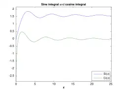
Intégrales trigonométriques
Si(x ) (bleu) et Ci(x ) (vert).
Sinus intégral
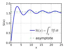
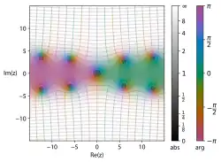
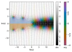
Tracé de Si(x ) pour 0 ≤ x ≤ 8 π . Sinus intégral sur le plan complexe, tracé avec une coloration de régions . Il existe deux fonctions sinus intégrales :
Si
(
x
)
=
∫
0
x
sin
t
t
d
t
{\displaystyle \operatorname {Si} (x)=\int _{0}^{x}{\frac {\sin t}{t}}\,\mathrm {d} t}
si
(
x
)
=
−
∫
x
∞
sin
t
t
d
t
.
{\displaystyle \operatorname {si} (x)=-\int _{x}^{\infty }{\frac {\sin t}{t}}\,\mathrm {d} t~.}
On peut remarquer que l'intégrande sin(t )/t est la fonction sinus cardinal , et la fonction de Bessel sphérique d'ordre 0.
Puisque sinc est une fonction entière paire (holomorphe sur tout le plan complexe), Si est entière, impaire, et l'intégrale dans sa définition peut être calculée le long de tout chemin reliant les extrémités.
Par définition, Si(x ) et la primitive de sin x / x qui s'annule en x = 0si(x ) est celle qui s'annule pour x → ∞intégrale de Dirichlet :
Si
(
x
)
−
si
(
x
)
=
∫
0
∞
sin
t
t
d
t
=
π
2
.
{\displaystyle \operatorname {Si} (x)-\operatorname {si} (x)=\int _{0}^{\infty }{\frac {\sin t}{t}}\,\mathrm {d} t={\frac {\pi }{2}}.}
En traitement du signal , les oscillations du sinus intégral génèrent des suroscillations en utilisant le filtre sinus cardinal, et des suroscillations fréquentielles en utilisant un filtre sinus cardinal tronqué comme filtre passe-bas .
Ce phénomène est en lien avec le phénomène de Gibbs : si le sinus intégral est considéré comme la convolution de la fonction sinus cardinal avec la fonction de Heaviside , cela revient à tronquer la série de Fourier , d'où l'apparition du phénomène de Gibbs.
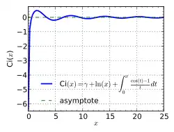
Cosinus intégral
Tracé de Ci(x ) pour 0 < x ≤ 8π . Tracé de Ci(x ) sur le plan complexe entre -2-2i et 2+2i . Cosinus intégral sur le plan complexe. On peut voir la coupure le long du demi-axe des réels négatifs. Il existe deux fonctions cosinus intégrales :
Ci
(
x
)
=
−
∫
x
∞
cos
t
t
d
t
{\displaystyle \operatorname {Ci} (x)=-\int _{x}^{\infty }{\frac {\cos t}{t}}\,\mathrm {d} t}
Cin
(
x
)
=
∫
0
x
1
−
cos
t
t
d
t
=
γ
+
ln
x
−
Ci
(
x
)
pour
|
Arg
(
x
)
|
<
π
,
{\displaystyle \operatorname {Cin} (x)=\int _{0}^{x}{\frac {1-\cos t}{t}}\,\mathrm {d} t=\gamma +\ln x-\operatorname {Ci} (x)\qquad ~{\text{ pour }}~\left|\operatorname {Arg} (x)\right|<\pi ~,}
où γ ≈ 0.57721566 ...constante d'Euler-Mascheroni . Certains textes utilisent la notation ci au lieu de Ci .
Ci(x ) est la primitive de cos(x )/x qui s'annule pour x → ∞
Cin est une fonction entière paire . Pour cela, certains auteurs préfèrent définir Cin puis en déduire Ci .
Généralisations
x réel positif, par[ 1]
∀
z
∈
C
,
0
<
ℜ
(
z
)
<
2
,
S
i
(
x
,
z
)
=
∫
0
x
sin
(
t
)
t
z
d
t
,
{\displaystyle \forall z\in \mathbb {C} ,\ 0<\Re (z)<2,\ \mathrm {Si} (x,z)=\int _{0}^{x}{\frac {\sin(t)}{t^{z}}}~\mathrm {d} t,}
∀
z
∈
C
,
0
<
ℜ
(
z
)
<
1
,
C
i
(
x
,
z
)
=
∫
0
x
cos
(
t
)
t
z
d
t
{\displaystyle \forall z\in \mathbb {C} ,\ 0<\Re (z)<1,\ \mathrm {Ci} (x,z)=\int _{0}^{x}{\frac {\cos(t)}{t^{z}}}~\mathrm {d} t}
On a alors :
S
i
(
x
,
0
)
=
1
−
cos
(
x
)
,
C
i
(
x
,
0
)
=
sin
(
x
)
{\displaystyle \mathrm {Si} (x,0)=1-\cos(x),\ \mathrm {Ci} (x,0)=\sin(x)}
S
i
(
x
,
1
)
=
S
i
(
x
)
,
C
i
(
x
,
1
)
=
∫
0
+
i
n
f
t
y
cos
(
t
)
t
z
d
t
−
C
i
(
x
)
{\displaystyle \mathrm {Si} (x,1)=\mathrm {Si} (x),\ \mathrm {Ci} (x,1)=\int _{0}^{+infty}{\frac {\cos(t)}{t^{z}}}~\mathrm {d} t-\mathrm {Ci} (x)}
S
i
(
x
,
1
/
2
)
=
2
S
(
x
)
,
C
i
(
x
,
1
/
2
)
=
2
C
(
x
)
{\displaystyle \mathrm {Si} (x,1/2)=2S({\sqrt {x}}),\,\mathrm {Ci} (x,1/2)=2C({\sqrt {x}})}
S et C sont les fonctions de Fresnel .Ces fonctions ont été utilisées dans l'étude du phénomène de Gibbs .
Relation avec l'exponentielle intégrale d'argument imaginaire
On considère la fonction exponentielle intégrale
E
1
(
z
)
=
∫
1
∞
exp
(
−
z
t
)
t
d
t
pour
ℜ
(
z
)
≥
0.
{\displaystyle \operatorname {E} _{1}(z)=\int _{1}^{\infty }{\frac {\exp(-zt)}{t}}\,\mathrm {d} t\qquad ~{\text{ pour }}~\Re (z)\geq 0.}
Si et Ci :
E
1
(
i
x
)
=
i
(
−
π
2
+
Si
(
x
)
)
−
Ci
(
x
)
=
i
si
(
x
)
−
ci
(
x
)
pour
x
>
0
.
{\displaystyle \operatorname {E} _{1}(\mathrm {i} x)=\mathrm {i} \left(-{\frac {\pi }{2}}+\operatorname {Si} (x)\right)-\operatorname {Ci} (x)=\mathrm {i} \operatorname {si} (x)-\operatorname {ci} (x)\qquad ~{\text{ pour }}~x>0~.}
Comme toutes ces fonctions sont analytiques sauf sur la branche des valeurs négatives de l'argument, le domaine de validité de la relation doit être étendu à (hors de ce domaine, des termes additionnels sous forme de facteurs entiers de π
Les cas de l'argument imaginaire pur de la fonction exponentielle intégrale sont
∫
1
∞
cos
(
a
x
)
ln
x
x
d
x
=
−
π
2
24
+
γ
(
γ
2
+
ln
a
)
+
ln
2
a
2
+
∑
n
≥
1
(
−
a
2
)
n
(
2
n
)
!
(
2
n
)
2
,
{\displaystyle \int _{1}^{\infty }\cos(ax){\frac {\ln x}{x}}\,\mathrm {d} x=-{\frac {\pi ^{2}}{24}}+\gamma \left({\frac {\gamma }{2}}+\ln a\right)+{\frac {\ln ^{2}a}{2}}+\sum _{n\geq 1}{\frac {(-a^{2})^{n}}{(2n)!\,(2n)^{2}}}~,}
partie réelle de
∫
1
∞
e
i
a
x
ln
x
x
d
x
=
−
π
2
24
+
γ
(
γ
2
+
ln
a
)
+
ln
2
a
2
−
π
2
i
(
γ
+
ln
a
)
+
∑
n
≥
1
(
i
a
)
n
n
!
n
2
.
{\displaystyle \int _{1}^{\infty }\mathrm {e} ^{\mathrm {i} ax}{\frac {\ln x}{x}}\,\mathrm {d} x=-{\frac {\pi ^{2}}{24}}+\gamma \left({\frac {\gamma }{2}}+\ln a\right)+{\frac {\ln ^{2}a}{2}}-{\frac {\pi }{2}}\mathrm {i} \left(\gamma +\ln a\right)+\sum _{n\geq 1}{\frac {(\mathrm {i} a)^{n}}{n!\,n^{2}}}~.}
De façon similaire,
∫
1
∞
e
i
a
x
ln
x
x
2
d
x
=
1
+
i
a
[
−
π
2
24
+
γ
(
γ
2
+
ln
a
−
1
)
+
ln
2
a
2
−
ln
a
+
1
]
+
π
a
2
(
γ
+
ln
a
−
1
)
+
∑
n
≥
1
(
i
a
)
n
+
1
(
n
+
1
)
!
n
2
.
{\displaystyle \int _{1}^{\infty }\mathrm {e} ^{\mathrm {i} ax}{\frac {\ln x}{x^{2}}}\,\mathrm {d} x=1+\mathrm {i} a\left[-{\frac {\pi ^{2}}{24}}+\gamma \left({\frac {\gamma }{2}}+\ln a-1\right)+{\frac {\ln ^{2}a}{2}}-\ln a+1\right]+{\frac {\pi a}{2}}\left(\gamma +\ln a-1\right)+\sum _{n\geq 1}{\frac {(\mathrm {i} a)^{n+1}}{(n+1)!\,n^{2}}}~.}
Méthodes de calcul efficaces
Les approximants de Padé des séries de Taylor convergentes donnent une méthode efficace d'évaluation des fonctions pour de petits arguments. Les formules suivantes, données par Rowe et al. (2015)[ 3] 10−16 pour 0 ≤ x ≤ 4 ,
Si
(
x
)
≈
x
⋅
(
1
−
4
,
54393409816329991
⋅
10
−
2
⋅
x
2
+
1
,
15457225751016682
⋅
10
−
3
⋅
x
4
−
1
,
41018536821330254
⋅
10
−
5
⋅
x
6
+
9
,
43280809438713025
⋅
10
−
8
⋅
x
8
−
3
,
53201978997168357
⋅
10
−
10
⋅
x
10
+
7
,
08240282274875911
⋅
10
−
13
⋅
x
12
−
6
,
05338212010422477
⋅
10
−
16
⋅
x
14
1
+
1
,
01162145739225565
⋅
10
−
2
⋅
x
2
+
4
,
99175116169755106
⋅
10
−
5
⋅
x
4
+
1
,
55654986308745614
⋅
10
−
7
⋅
x
6
+
3
,
28067571055789734
⋅
10
−
10
⋅
x
8
+
4
,
5049097575386581
⋅
10
−
13
⋅
x
10
+
3
,
21107051193712168
⋅
10
−
16
⋅
x
12
)
Ci
(
x
)
≈
γ
+
ln
(
x
)
+
x
2
⋅
(
−
0
,
25
+
7
,
51851524438898291
⋅
10
−
3
⋅
x
2
−
1
,
27528342240267686
⋅
10
−
4
⋅
x
4
+
1
,
05297363846239184
⋅
10
−
6
⋅
x
6
−
4
,
68889508144848019
⋅
10
−
9
⋅
x
8
+
1
,
06480802891189243
⋅
10
−
11
⋅
x
10
−
9
,
93728488857585407
⋅
10
−
15
⋅
x
12
1
+
1
,
1592605689110735
⋅
10
−
2
⋅
x
2
+
6
,
72126800814254432
⋅
10
−
5
⋅
x
4
+
2
,
55533277086129636
⋅
10
−
7
⋅
x
6
+
6
,
97071295760958946
⋅
10
−
10
⋅
x
8
+
1
,
38536352772778619
⋅
10
−
12
⋅
x
10
+
1
,
89106054713059759
⋅
10
−
15
⋅
x
12
+
1
,
39759616731376855
⋅
10
−
18
⋅
x
14
)
{\displaystyle {\begin{array}{rcl}\operatorname {Si} (x)&\approx &x\cdot \left({\frac {\begin{array}{l}1-4,54393409816329991\cdot 10^{-2}\cdot x^{2}+1,15457225751016682\cdot 10^{-3}\cdot x^{4}-1,41018536821330254\cdot 10^{-5}\cdot x^{6}\\~~~+9,43280809438713025\cdot 10^{-8}\cdot x^{8}-3,53201978997168357\cdot 10^{-10}\cdot x^{10}+7,08240282274875911\cdot 10^{-13}\cdot x^{12}\\~~~-6,05338212010422477\cdot 10^{-16}\cdot x^{14}\end{array}}{\begin{array}{l}1+1,01162145739225565\cdot 10^{-2}\cdot x^{2}+4,99175116169755106\cdot 10^{-5}\cdot x^{4}+1,55654986308745614\cdot 10^{-7}\cdot x^{6}\\~~~+3,28067571055789734\cdot 10^{-10}\cdot x^{8}+4,5049097575386581\cdot 10^{-13}\cdot x^{10}+3,21107051193712168\cdot 10^{-16}\cdot x^{12}\end{array}}}\right)\\&~&\\\operatorname {Ci} (x)&\approx &\gamma +\ln(x)+x^{2}\cdot \left({\frac {\begin{array}{l}-0,25+7,51851524438898291\cdot 10^{-3}\cdot x^{2}-1,27528342240267686\cdot 10^{-4}\cdot x^{4}+1,05297363846239184\cdot 10^{-6}\cdot x^{6}\\~~~-4,68889508144848019\cdot 10^{-9}\cdot x^{8}+1,06480802891189243\cdot 10^{-11}\cdot x^{10}-9,93728488857585407\cdot 10^{-15}\cdot x^{12}\\\end{array}}{\begin{array}{l}1+1,1592605689110735\cdot 10^{-2}\cdot x^{2}+6,72126800814254432\cdot 10^{-5}\cdot x^{4}+2,55533277086129636\cdot 10^{-7}\cdot x^{6}\\~~~+6,97071295760958946\cdot 10^{-10}\cdot x^{8}+1,38536352772778619\cdot 10^{-12}\cdot x^{10}+1,89106054713059759\cdot 10^{-15}\cdot x^{12}\\~~~+1,39759616731376855\cdot 10^{-18}\cdot x^{14}\\\end{array}}}\right)\end{array}}}
Les intégrales peuvent également être évaluées indirectement par les fonctions auxiliaires
f
(
x
)
{\displaystyle f(x)}
g
(
x
)
{\displaystyle g(x)}
Pour x ≥ 4, les fonctions rationnelles de Padé ci-dessous approchent
f
(
x
)
{\displaystyle f(x)}
g
(
x
)
{\displaystyle g(x)}
10−16 [ 3]
f
(
x
)
≈
1
x
⋅
(
1
+
7
,
44437068161936700618
⋅
10
2
⋅
x
−
2
+
1
,
96396372895146869801
⋅
10
5
⋅
x
−
4
+
2
,
37750310125431834034
⋅
10
7
⋅
x
−
6
+
1
,
43073403821274636888
⋅
10
9
⋅
x
−
8
+
4
,
33736238870432522765
⋅
10
10
⋅
x
−
10
+
6
,
40533830574022022911
⋅
10
11
⋅
x
−
12
+
4
,
20968180571076940208
⋅
10
12
⋅
x
−
14
+
1
,
00795182980368574617
⋅
10
13
⋅
x
−
16
+
4
,
94816688199951963482
⋅
10
12
⋅
x
−
18
−
4
,
94701168645415959931
⋅
10
11
⋅
x
−
20
1
+
7
,
46437068161927678031
⋅
10
2
⋅
x
−
2
+
1
,
97865247031583951450
⋅
10
5
⋅
x
−
4
+
2
,
41535670165126845144
⋅
10
7
⋅
x
−
6
+
1
,
47478952192985464958
⋅
10
9
⋅
x
−
8
+
4
,
58595115847765779830
⋅
10
10
⋅
x
−
10
+
7
,
08501308149515401563
⋅
10
11
⋅
x
−
12
+
5
,
06084464593475076774
⋅
10
12
⋅
x
−
14
+
1
,
43468549171581016479
⋅
10
13
⋅
x
−
16
+
1
,
11535493509914254097
⋅
10
13
⋅
x
−
18
)
g
(
x
)
≈
1
x
2
⋅
(
1
+
8
,
1359520115168615
⋅
10
2
⋅
x
−
2
+
2
,
35239181626478200
⋅
10
5
⋅
x
−
4
+
3
,
12557570795778731
⋅
10
7
⋅
x
−
6
+
2
,
06297595146763354
⋅
10
9
⋅
x
−
8
+
6
,
83052205423625007
⋅
10
10
⋅
x
−
10
+
1
,
09049528450362786
⋅
10
12
⋅
x
−
12
+
7
,
57664583257834349
⋅
10
12
⋅
x
−
14
+
1
,
81004487464664575
⋅
10
13
⋅
x
−
16
+
6
,
43291613143049485
⋅
10
12
⋅
x
−
18
−
1
,
36517137670871689
⋅
10
12
⋅
x
−
20
1
+
8
,
19595201151451564
⋅
10
2
⋅
x
−
2
+
2
,
40036752835578777
⋅
10
5
⋅
x
−
4
+
3
,
26026661647090822
⋅
10
7
⋅
x
−
6
+
2
,
23355543278099360
⋅
10
9
⋅
x
−
8
+
7
,
87465017341829930
⋅
10
10
⋅
x
−
10
+
1
,
39866710696414565
⋅
10
12
⋅
x
−
12
+
1
,
7164723371736605
⋅
10
13
⋅
x
−
14
+
4
,
01839087307656620
⋅
10
13
⋅
x
−
16
+
3
,
99653257887490811
⋅
10
13
⋅
x
−
18
)
{\displaystyle {\begin{array}{rcl}f(x)&\approx &{\dfrac {1}{x}}\cdot \left({\frac {\begin{array}{l}1+7,44437068161936700618\cdot 10^{2}\cdot x^{-2}+1,96396372895146869801\cdot 10^{5}\cdot x^{-4}+2,37750310125431834034\cdot 10^{7}\cdot x^{-6}\\~~~+1,43073403821274636888\cdot 10^{9}\cdot x^{-8}+4,33736238870432522765\cdot 10^{10}\cdot x^{-10}+6,40533830574022022911\cdot 10^{11}\cdot x^{-12}\\~~~+4,20968180571076940208\cdot 10^{12}\cdot x^{-14}+1,00795182980368574617\cdot 10^{13}\cdot x^{-16}+4,94816688199951963482\cdot 10^{12}\cdot x^{-18}\\~~~-4,94701168645415959931\cdot 10^{11}\cdot x^{-20}\end{array}}{\begin{array}{l}1+7,46437068161927678031\cdot 10^{2}\cdot x^{-2}+1,97865247031583951450\cdot 10^{5}\cdot x^{-4}+2,41535670165126845144\cdot 10^{7}\cdot x^{-6}\\~~~+1,47478952192985464958\cdot 10^{9}\cdot x^{-8}+4,58595115847765779830\cdot 10^{10}\cdot x^{-10}+7,08501308149515401563\cdot 10^{11}\cdot x^{-12}\\~~~+5,06084464593475076774\cdot 10^{12}\cdot x^{-14}+1,43468549171581016479\cdot 10^{13}\cdot x^{-16}+1,11535493509914254097\cdot 10^{13}\cdot x^{-18}\end{array}}}\right)\\&&\\g(x)&\approx &{\dfrac {1}{x^{2}}}\cdot \left({\frac {\begin{array}{l}1+8,1359520115168615\cdot 10^{2}\cdot x^{-2}+2,35239181626478200\cdot 10^{5}\cdot x^{-4}+3,12557570795778731\cdot 10^{7}\cdot x^{-6}\\~~~+2,06297595146763354\cdot 10^{9}\cdot x^{-8}+6,83052205423625007\cdot 10^{10}\cdot x^{-10}+1,09049528450362786\cdot 10^{12}\cdot x^{-12}\\~~~+7,57664583257834349\cdot 10^{12}\cdot x^{-14}+1,81004487464664575\cdot 10^{13}\cdot x^{-16}+6,43291613143049485\cdot 10^{12}\cdot x^{-18}\\~~~-1,36517137670871689\cdot 10^{12}\cdot x^{-20}\end{array}}{\begin{array}{l}1+8,19595201151451564\cdot 10^{2}\cdot x^{-2}+2,40036752835578777\cdot 10^{5}\cdot x^{-4}+3,26026661647090822\cdot 10^{7}\cdot x^{-6}\\~~~+2,23355543278099360\cdot 10^{9}\cdot x^{-8}+7,87465017341829930\cdot 10^{10}\cdot x^{-10}+1,39866710696414565\cdot 10^{12}\cdot x^{-12}\\~~~+1,7164723371736605\cdot 10^{13}\cdot x^{-14}+4,01839087307656620\cdot 10^{13}\cdot x^{-16}+3,99653257887490811\cdot 10^{13}\cdot x^{-18}\end{array}}}\right)\\\end{array}}}


_in_the_complex_plane_from_-2-2i_to_2%252B2i_with_colors_created_with_Mathematica_13.1_function_ComplexPlot3D.svg.png)


_in_the_complex_plane_from_-2-2i_to_2%252B2i_with_colors_created_with_Mathematica_13.1_function_ComplexPlot3D.svg.png)


_in_the_complex_plane_from_-2-2i_to_2%252B2i_with_colors_created_with_Mathematica_13.1_function_ComplexPlot3D.svg.png)


![{\displaystyle {\begin{aligned}f(x)\equiv &\int _{0}^{\infty }{\frac {\sin(t)}{t+x}}\,\mathrm {d} t&=&\int _{0}^{\infty }{\frac {\mathrm {e} ^{-xt}}{t^{2}+1}}\,\mathrm {d} t&=&\operatorname {Ci} (x)\sin(x)+\left[{\frac {\pi }{2}}-\operatorname {Si} (x)\right]\cos(x)~,\\[5pt]g(x)\equiv &\int _{0}^{\infty }{\frac {\cos(t)}{t+x}}\,\mathrm {d} t&=&\int _{0}^{\infty }{\frac {t\mathrm {e} ^{-xt}}{t^{2}+1}}\,\mathrm {d} t&=&-\operatorname {Ci} (x)\cos(x)+\left[{\frac {\pi }{2}}-\operatorname {Si} (x)\right]\sin(x)~.\end{aligned}}}](./ea60947c6d639f2550728c1feb5a58ff360692dc.svg)


![{\displaystyle \int _{1}^{\infty }\mathrm {e} ^{\mathrm {i} ax}{\frac {\ln x}{x^{2}}}\,\mathrm {d} x=1+\mathrm {i} a\left[-{\frac {\pi ^{2}}{24}}+\gamma \left({\frac {\gamma }{2}}+\ln a-1\right)+{\frac {\ln ^{2}a}{2}}-\ln a+1\right]+{\frac {\pi a}{2}}\left(\gamma +\ln a-1\right)+\sum _{n\geq 1}{\frac {(\mathrm {i} a)^{n+1}}{(n+1)!\,n^{2}}}~.}](./fad479e819d78322c9ce8f675cfc25a7e2f35667.svg)


 Portail de l'analyse